


I benchmarked 9 implementations across 7 AI approaches for streaming classification on Kafka — 5,000 real UK procurement tenders, same stream, same clock. Accuracy, latency, and cost compared across hardcoded rules, constraint solvers, ONNX ML, LangChain, n8n, and MCP.
Nine AI Paradigms. One Kafka Stream. First Numbers.
I built nine AI approaches for one simple task: classify UK public procurement contracts into 34 CPV categories.
Same 5,000 records. Same ground truth. Same live Kafka stream.
No notebook benchmark. Each consumer read from Confluent Cloud. Each result landed in PostgreSQL. The classifiers never saw the true category.
I measured three things:
- accuracy;
- latency per record;
- cost per run.
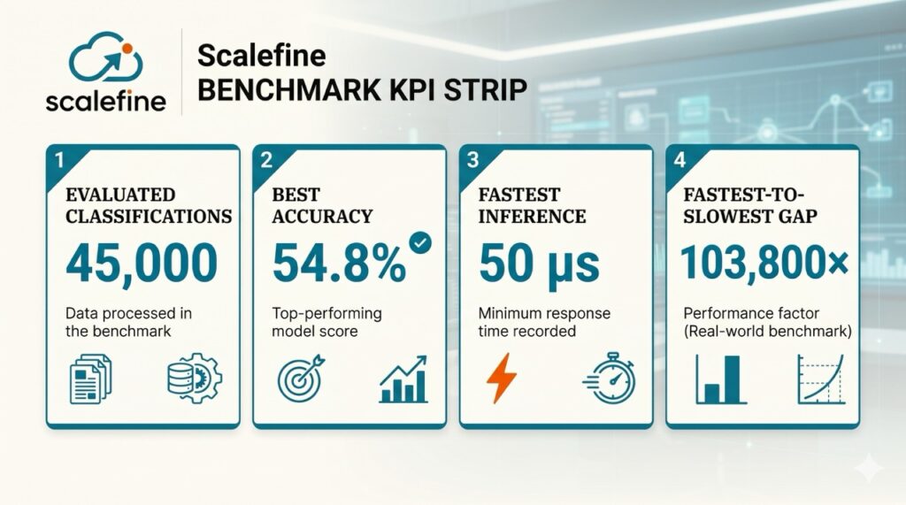
The fastest model processed one record in 50 µs.
The slowest took 5,190 ms.
That is a 103,800× gap on the same classification task.
This is not a verdict on LLMs, MCP, rules, or trained ML.
It is the baseline.
Classification is deliberately simple. Inputs are bounded. The expected answer already exists. That makes it a clean first test for a real-time pipeline.
The next benchmark will use the same nine paradigms on harder work: structured output generation, multi-source reconciliation, and multi-step reasoning.
That is where LLMs and agentic systems should start earning their complexity.
But first: the numbers on the easy case.
If you do not have evals, you do not know whether you are moving the needle.
The Test Bed: From Tender Text to Spend Visibility
A tender is a public buyer describing a need and inviting suppliers to compete for it. In the UK, a buyer publishes an opportunity, suppliers bid, the buyer evaluates them, and one supplier receives the contract.
UK Contracts Finder exposes those records as public data. Each one includes a tender_title and a tender_description. Some are detailed. Some are barely more than “IT support services”.
The task was to assign one CPV category to each tender. CPV is the Common Procurement Vocabulary. I used the two-digit level: 45 for construction, 72 for IT services, 85 for health, 30 for office equipment. One tender. One category. 34 possible outputs.
I could have simply used the existing category mapping. The dataset already contains the real CPV code in tender_classification_id.
That would have defeated the point.
The exercise was to see whether nine very different AI approaches could infer the category from the tender text alone. The real CPV code stayed hidden during classification and became the source of truth afterwards, when I calculated accuracy.
This is the data layer behind spend analytics. Once contracts are consistently classified, you can group spend by category, supplier, business unit, geography, or period. That is the kind of visibility shown in Oracle Fusion ERP Analytics Spend Analytics: where money goes, which categories grow, and where purchasing fragments.
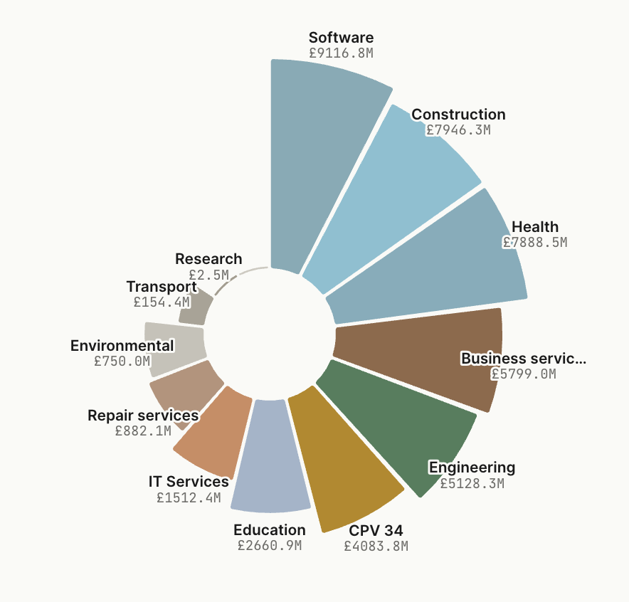
I loaded 47,733 UK procurement records into Kafka and used the first 5,000 for this benchmark. The remaining ~42,733 stayed untouched. Every approach started from the same Kafka offset and wrote predictions to local PostgreSQL.
The setup was simple: a MacBook Air M4 with 16 GB RAM in Bangkok, Confluent Cloud Basic in Singapore, one cpv-raw topic, and nine consumer groups. Latency covered the classification call only. Not Kafka polling, database writes, or network delay.
For trained ML models, even-indexed records trained the model. Odd-indexed records remained unseen. All 5,000 still appeared in the final score. LLM, rule-based, and solver approaches received no training data.
Each paradigm got one hour maximum for implementation and optimisation. Most took closer to 30 minutes.
Simple on purpose. You need the floor before you measure the ceiling.
This is also how I start client work when an AI or streaming decision is still unclear.
Not with a slide deck. With a small, time-boxed proof on the real data, the real throughput, and the real delivery constraints.
Sometimes the result is “use the LLM.” Sometimes it is “keep the rules.” Both answers are cheaper than six months of architecture theatre.
Nine (AI) Ways to Classify the Same Tender
These nine approaches range from keyword matching to agentic LLM workflows.
They do not solve the same kind of problem equally well. That is exactly why I put them on the same stream.
1. Hardcoded Rules: A Very Organised CTRL+F
The simplest approach used no AI at all.
I created a dictionary of CPV categories and associated keywords. Words such as “construction”, “building”, or “highway” pushed a tender towards category 45. The title counted three times more than the description because it is usually cleaner.
This is fast, cheap, auditable, and runs offline. It is also blind to meaning. “Support” can mean IT support, social care support, or construction support.
It reached 29.4% accuracy. Better than random. But keyword matching has a natural ceiling.
2. Constraint Solver: Rules With a Referee
The hardcoded version counts keywords and picks the highest score.
The solver adds a referee.
I defined every CPV category in a small domain language. Each rule can contain positive signals, numerical conditions, hard exclusions, and a fallback priority.
A simplified construction rule looked like this:
CATEGORY 45 "Construction":
    soft  construction*3, building*2, civil*2, refurbishment*2, highway*2
    soft  value_gbp >= 250_000 : +2
    hard  NOT (software OR licence)
    prior 1.0
The soft lines add evidence. “Highway” or “refurbishment” pushes the tender towards construction.
The value condition adds a small extra signal above £250,000. Useful, but never enough on its own.
The hard line is different. Mention “software” or “licence”, and category 45 is removed completely.
The prior only breaks a tie.
Z3 solver compares every valid category, removes the impossible ones, then selects the strongest remaining match.
This is useful when rules must be explicit and auditable. Think compliance, eligibility, or any decision where “why did this happen?” needs a precise answer.
It reached 30.1% accuracy. Plain keyword matching reached 29.4%.
I also tested more elaborate combinations and penalties. They helped on clean examples, then failed on messy tender language.
That is the symbolic ceiling here. Rules formalise known signals. They do not learn new language patterns.
3. Random Forest + Embeddings: 100 Small Voters
This was the strongest trained ML approach.
A Random Forest is classic machine learning. It builds many small decision trees from labelled examples. Each tree makes a category choice. The forest takes the majority vote.
But trees do not read text.
First, each tender had to become an embedding: a list of numbers that captures what the text is about. Similar tenders should end up close together in that numerical space. The Random Forest then learns which regions tend to map to construction, IT, health, or another CPV category.
I tested two embedding models.
Model2Vec (minishlab/potion-base-8M) uses lightweight static vectors. It is closer to a very smart bag of words: each token has a fixed representation, then the model combines them. It loses some context, but it is extremely fast.
MiniLM (all-MiniLM-L6-v2) is a small transformer. It reads the sentence as a whole, so the same word can mean different things depending on its context. That usually gives richer signals, but costs more latency.
Both embedding models and the Random Forest ran through ONNX with onnxruntime. No PyTorch. No Transformers runtime. Just portable inference.
MiniLM + Random Forest reached 54.4% accuracy at 58.9 ms per record.
Model2Vec + Random Forest reached 53.4% at 0.06 ms.
That is a 0.4-point accuracy gap for a 983× latency gap.
4. Deep Learning + Embeddings: A Neural Network Instead of a Forest
The deep-learning variants used the same embeddings, but replaced the Random Forest with a small neural network.
The model was a simple MLP: two dense layers, ReLU, and dropout. It trained for 25 epochs, then exported to ONNX for inference.
This approach can learn more complex boundaries when enough labelled examples exist. With roughly 2,500 training records, it did not beat the Random Forest here.
MiniLM + MLP reached 51.3%.
Model2Vec + MLP reached 48.8%.
The lesson is not “deep learning is worse”. The lesson is that model capacity is useless when the dataset is small or the problem does not need it.
5. LangChain + Gemini: A Generalist With No Training Data
A Large Language Model is a model trained beforehand on huge amounts of text. ChatGPT from OpenAI, Claude from Anthropic, and Gemini from Google are the best-known examples.
They do not need a custom model for every task. You give them instructions, context, and a required output. They use general language knowledge to produce an answer.
For each tender, I sent Gemini 2.5 Flash Lite the 34 CPV categories, the title, and the description. Then I asked for one two-digit code. Nothing else.
This is zero-shot classification. No training examples. No fine-tuning. No procurement-specific model.
LangChain handled the plumbing: build the prompt, call the Gemini API, validate the returned code, and run eight requests in parallel.
That pattern is already used in real businesses. Intercom uses Claude in its Fin support agent to resolve customer queries. 7-Eleven Vietnam uses Gemini in an internal assistant that helps store employees resolve IT issues. The common pattern is simple: take unstructured language, add relevant context, then return a useful answer.
This works well when you have no labelled data, the labels are ambiguous, or vocabulary changes faster than you can retrain a model.
In our experiment it reached the highest accuracy: 54.8%.
It also took 2,148 ms per record. Most of that time came from the API round trip and text generation.
6. n8n + Gemini: The Same Model, Routed Through a Workflow
n8n is a visual automation tool. Instead of writing every integration in code, you connect steps as boxes on a canvas.
In this version, Python sent each tender to an n8n webhook. n8n built the request, called Gemini, received the CPV code, then returned JSON.
The model and prompt strategy were the same as LangChain. The difference was operational: the workflow lived in n8n rather than in the application.
This is useful when operations, support, or business teams need to inspect and change a flow without opening a codebase. A typical workflow might receive a support ticket, ask Gemini to classify it, create a ticket in Jira, and notify the relevant team in Slack.
The trade-off is another system to run. The Python client was only 61 lines, but the flow added 131 lines of JSON and an n8n instance to host, secure, monitor, and debug.
It reached 45.3% accuracy at 3,039 ms per record.
7. MCP Agent: A Model That Can Ask for Tools
MCP stands for Model Context Protocol. It is a standard for letting models such as Claude, ChatGPT, or Gemini use external tools and data sources.
A normal LLM prompt is like giving someone a document and asking for an answer. An MCP-enabled model can also query a database, search a knowledge base, read a customer record, run a calculation, or trigger an action.
For this benchmark, Gemini had two tools. One listed CPV divisions. The other returned likely keywords for the current tender.
The model could decide which tool to call first, read the result, then call another tool if needed. I allowed up to three rounds before it returned its CPV code.
That is an agentic workflow. The model is not only answering. It is choosing how to gather information before answering.
This is where MCP starts to make sense in real companies. A support agent can retrieve an account status, search product documentation, then draft a reply. A finance agent can pull current data, calculate a variance, and prepare a report. A legal workflow can search contracts, extract clauses, and flag missing obligations.
For direct classification, my two tools did not add enough information to justify the extra rounds. This version reached 40.3% accuracy and took 5,190 ms per record.
That does not make MCP a bad approach. It makes it a poor fit for simple, high-volume classification.
The next benchmark will use the same setup on harder tasks, where tool calls should add real value.
The Leaderboard: Same Tender, Same Stream, Very Different Economics
Same task. Same 5,000 tenders. Same Kafka offset.
The table does not declare a universal winner.
It shows the trade-offs on one deliberately simple task.
| Approach | Accuracy | Latency / record | Total time / 5k | Marginal cost / 5k | Marginal cost / 1M |
|---|---|---|---|---|---|
| LangChain + Gemini | 54.8% | 2,148 ms | 31m 22s | ~$0.22 | ~$44.70 |
| Random Forest + MiniLM | 54.4% | 58.9 ms | 4m 53s | ~$0 | ~$0 |
| Random Forest + Model2Vec | 53.4% | 0.06 ms | 0.4s | ~$0 | ~$0 |
| Deep Learning + MiniLM | 51.3% | 61.2 ms | 5m 5s | ~$0 | ~$0 |
| Deep Learning + Model2Vec | 48.8% | 0.05 ms | 0.4s | ~$0 | ~$0 |
| n8n + Gemini | 45.3% | 3,039 ms | 42m 50s | ~$0.22 + n8n hosting | ~$44.70 + hosting |
| MCP + Gemini | 40.3% | 5,190 ms | 47m 11s | ~$1.26 | ~$252.50 |
| Constraint Solver + Z3 | 30.1% | 2.3 ms | 11.7s | ~$0 | ~$0 |
| Hardcoded Rules | 29.4% | 0.41 ms | 2.2s | ~$0 | ~$0 |
ML models trained on roughly 2,500 even-indexed records and were evaluated across all 5,000. LLM approaches were zero-shot across all 5,000. Rules and the solver received no training data.
Two details matter.
First: LangChain and Random Forest + MiniLM were effectively tied on accuracy. 54.8% versus 54.4%. One used a general-purpose LLM with no procurement training. The other used a trained classical ML model.
Second: Model2Vec + Random Forest gave up one accuracy point against MiniLM + Random Forest. In return, it reduced latency from 58.9 ms to 0.06 ms per record.
That is not a rounding error.
At one million tenders, it is roughly 16 hours versus one minute of classification time on this hardware.
The MCP number needs the right reading. Its higher token bill comes from repeated model-and-tool rounds. That is wasted work for a direct classification task. On a task that genuinely needs retrieval, reconciliation, or multi-step decisions, those rounds may be the whole point.
Three Things the Numbers Make Clear
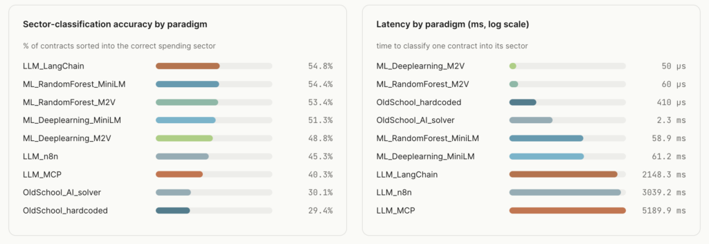
1. The Best LLM and the Best Trained ML Model Landed in the Same Range
LangChain + Gemini reached 54.8% accuracy.
Random Forest + MiniLM reached 54.4%.
That is 20 additional correct predictions across 5,000 tenders. A 0.4-point difference is too small to claim a meaningful winner here without a paired significance test.
The other LLM implementations were not close. n8n + Gemini reached 45.3%. MCP + Gemini reached 40.3%.
Gemini was zero-shot. It received no labelled procurement examples. The Random Forest trained on roughly 2,500 labelled tenders.
We did not fine-tune the LLM. We trained the Random Forest on ~2,500 examples. Same effort bracket, different approach.
The practical question is simple: do you already have labelled data? For bounded classification, a few thousand examples may be enough to reach the same accuracy range as a zero-shot LLM, with much lower latency and no token bill.
A fine-tuned LLM could change the result. I did not test that here. This was a comparison of realistic first implementations, not a fully optimised research project.
2. The Embedding Choice Was More Important Than the Classifier
Random Forest + MiniLM reached 54.4% at 58.9 ms per record.
Random Forest + Model2Vec reached 53.4% at 0.06 ms.
Same classifier. Same training records. Same categories. Only the embedding changed.
MiniLM is a small transformer. It reads the text as a sequence and produces a context-aware representation.
Model2Vec uses lightweight static vectors. It captures less context, but skips transformer inference entirely.
The result was a 983× latency gap for one accuracy point. At one million records, Model2Vec would take roughly one minute on this hardware. MiniLM would take roughly 16 hours.
For this streaming classification task, the embedding choice mattered more than whether the classifier was a Random Forest or a neural network.
3. Complexity Has a Price — But Only Relative to the Task
MCP was the most flexible LLM setup. Gemini could call tools, inspect their output, then decide whether to make another call before returning a category.
That is useful for retrieval, cross-system checks, calculations, and multi-step decisions. For direct classification, the tools added rounds without adding enough signal.
MCP reached 40.3% accuracy and took 47 minutes for 5,000 tenders. It required a tool server, async concurrency, and up to three model-tool rounds per record.
n8n used a more fixed workflow: receive the tender, call Gemini, return a CPV code. It was less flexible than MCP, but reached 45.3% accuracy and took 42 minutes 50 seconds.
Its value is operational, not raw speed. A business team can inspect or modify a stable workflow without changing application code: classify a support ticket, extract invoice fields, route an approval, notify a team.
The trade-off is that the complexity moves elsewhere. The Python client used 61 lines, but the workflow added 131 lines of JSON and an n8n instance to host, secure, monitor, and debug.
By contrast, Deep Learning + Model2Vec used around 40 lines of classifier code, needed no external service at inference, finished in 0.4 seconds, and reached 48.8% accuracy.
This does not make MCP or n8n bad choices. It shows what they cost on simple, high-volume classification.
This is usually where delivery gets stuck.
The prototype works. The cost model is unclear. Latency is ignored until traffic arrives. Or the workflow has become too complex for anyone to change safely.
Those are not “AI problems”. They are production engineering problems.
The next benchmark will test the same approaches on tasks where tool use and multi-step reasoning should add real value.
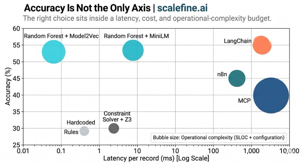
A Practical Decision Framework
The numbers are not a universal ranking.
They are a starting point for choosing an approach based on the task, the data you already have, and the latency budget you cannot violate.
| Approach | Use when | Avoid when |
|---|---|---|
| Hardcoded rules | Fewer than ~20 rules cover most cases. You need sub-millisecond latency, full auditability, offline execution, or zero infrastructure. | Categories overlap, wording changes often, or the text rarely contains obvious keywords. |
| Constraint solver / Z3 | Rules must combine safely. You need explicit exclusions, compliance logic, or a precise explanation for each decision. | You need semantic understanding from messy text, or you are processing very large volumes with a tight latency budget. |
| Trained ML + ONNX | You have a few thousand labelled examples, stable categories, and a strict latency or cost budget. | You have no training data, labels change frequently, or the task needs open-ended reasoning. |
| LLM via LangChain | You have little or no labelled data. Categories are ambiguous, wording evolves, or a general language model can add useful context. | You need high throughput, sub-second response times, or token cost matters at volume. |
| n8n + LLM | The workflow is stable and business teams need to inspect, edit, or connect it to other tools without changing application code. | The path is latency-sensitive, throughput is high, or an external workflow service adds more operational cost than value. |
| Agentic / MCP | The model must retrieve information, call tools, reconcile sources, calculate values, or reason across several steps. | The answer is directly available from one input and one classification pass. |
Start with the simplest approach that can meet the required accuracy.
Then measure it on your data.
A more capable approach is only better when the task actually needs the capability you are paying for.
If your team is stuck between “just ship the POC” and “rebuild the platform properly”, start by measuring the decision on your own workload.
That is the work I do: streaming data systems, AI paths from proof to production, and rescue work when a delivery has stopped moving.
This Was the Baseline, Not the Final Verdict
The full benchmark code, methodology, and UK Contracts Finder dataset pipeline are available in the spendlabel repository.
This was episode one: a deliberately simple classification task with known labels, fixed categories, and a clear latency budget.
The next benchmark will keep the same nine approaches, then move to a harder problem: structured output generation, multi-source reconciliation, or multi-step decisions with evidence.
That is where LLMs and agentic workflows should start to earn their extra cost and complexity.
Some rankings will probably flip.
The useful question is never “which AI approach is best?”
It is: does it work on your data, at your volume, inside your latency and cost constraints?
If that question is currently blocking a streaming or AI delivery, that is exactly the kind of problem I take on.